CS 180 NeRF Project

Project Overview

This project explores the implementation of Neural Radiance Fields (NeRF) to represent 2D images and 3D scenes. The project is divided into two parts: fitting a neural field to a 2D image and creating a NeRF for multi-view 3D scenes. Techniques like sinusoidal positional encoding, ray sampling, and volume rendering are used to build and optimize these models.

Part 1: Neural Field for 2D Image

In this part, a neural field is optimized to fit a 2D image. A multilayer perceptron (MLP) is used with sinusoidal positional encoding to learn the mapping from pixel coordinates to RGB values. The training process includes random pixel sampling and minimizing mean squared error loss.

The architecture used is the one below:

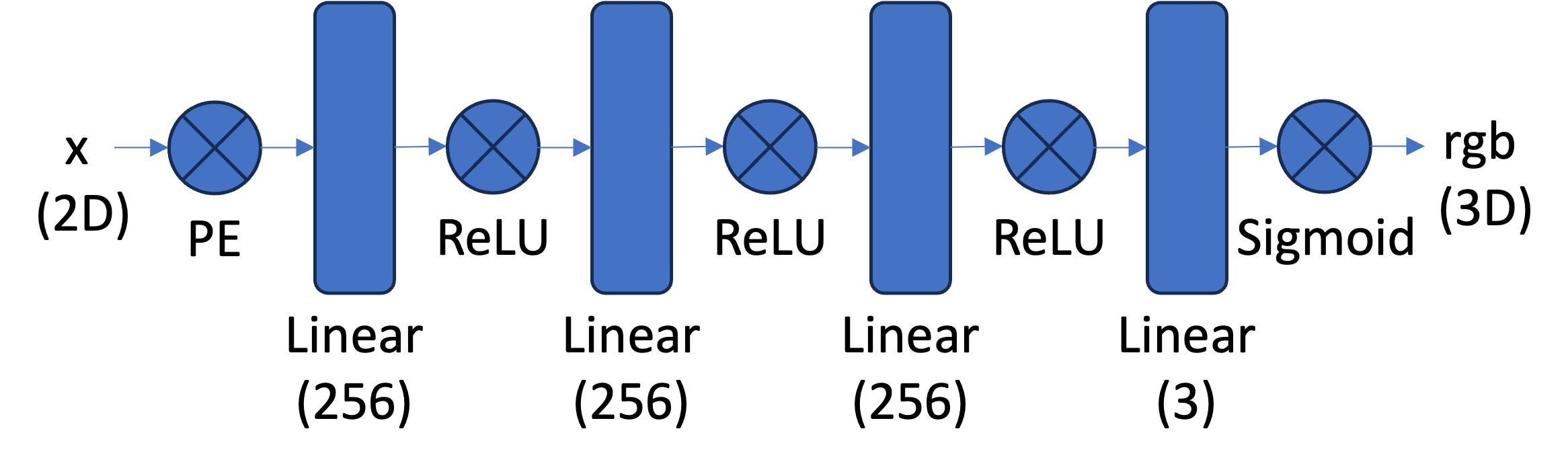
The hyperparameters we used were:

Number of layers: 4
Channel size: 256
Max frequency for the positional encoding: 10
Learning rate: 0.01
Batch Size: 10K
Number of Epochs: 10

Training Process Visualization

Iteration 10

Iteration 100

Iteration 500

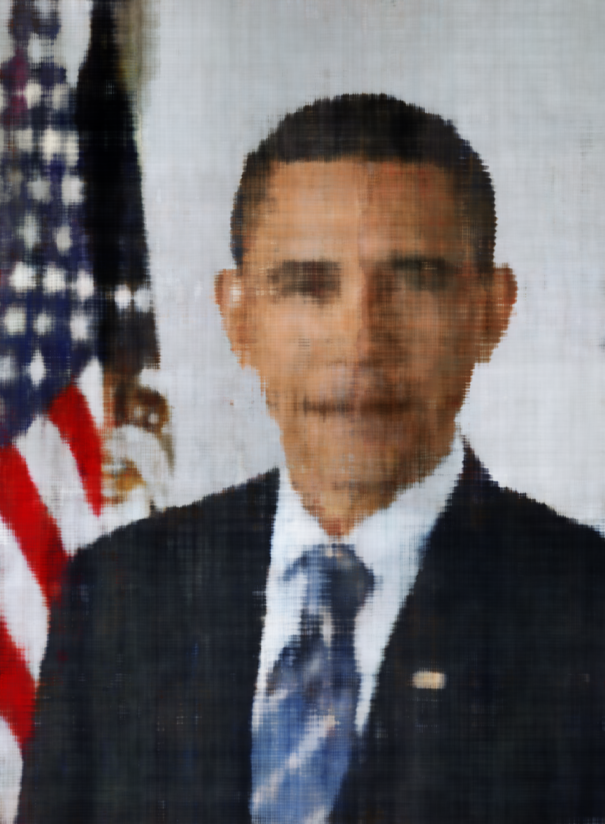
Iteration 800

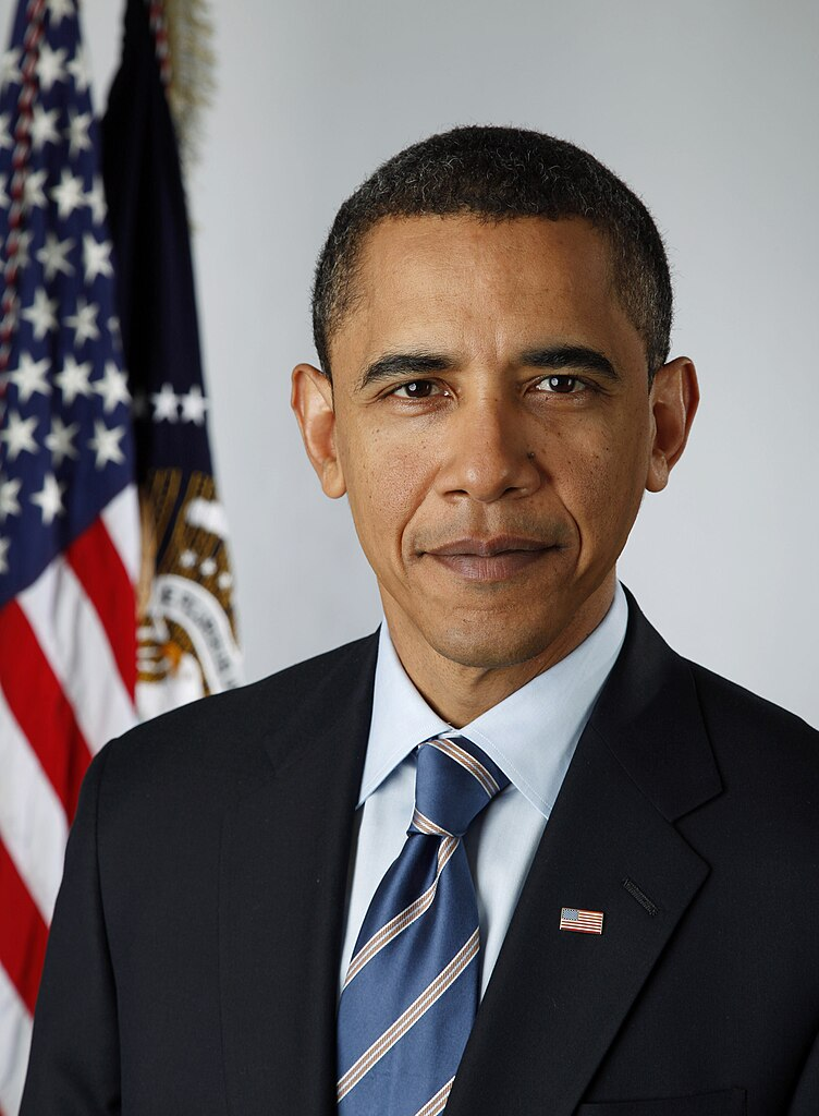
Original Image

Visualization of the predicted image across training iterations.

PSNR Curve for Obama

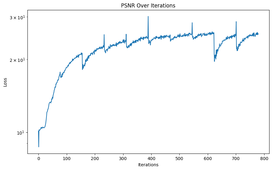
Plot showing the PSNR across training iterations for the picture of Obama. We can see that the PSNR has occassional spikes which don't appear in the fox PSNR curve.

Here is the image of the fox over iterations with the tasks hypersparameters and the original image.

Iteration 10

Iteration 100

Iteration 500

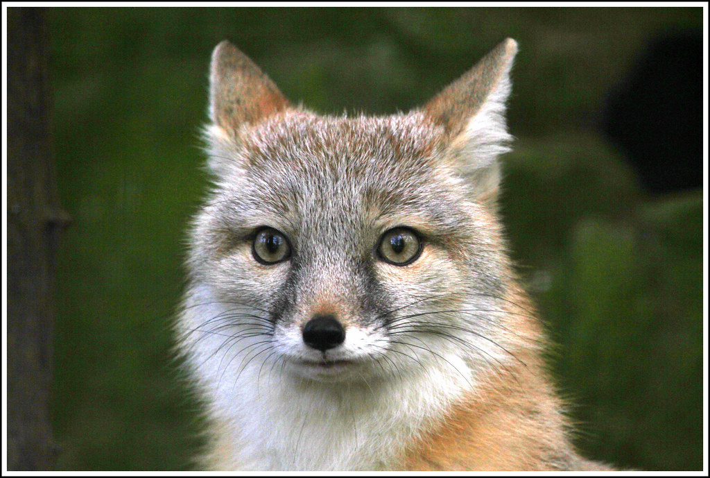
Original Image

PSNR Curve for the fox

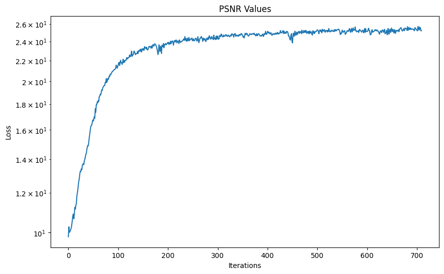
Plot showing the PSNR across training iterations for the Fox.

Part 2: Neural Radiance Field for 3D Scenes

Part 2.1: Create Rays from Cameras

Camera to World Coordinate Conversion

We implemented the camera-to-world coordinate transformation by defining a function x_w = transform(c2w, x_c), which converts points from the camera space to the world space. The inverse operation was also implemented to verify the correctness of the transformation. We used either NumPy or PyTorch for matrix multiplication, ensuring support for batched operations to handle multiple points efficiently.

Pixel to Camera Coordinate Conversion

To map pixel coordinates (u, v) to camera coordinates (x_c, y_c, z_c), we defined a function x_c = pixel_to_camera(K, uv, s), where K is the camera intrinsic matrix and s represents depth. This function was implemented to invert the projection process defined by the intrinsic matrix. We also added batch processing support for scalability during rendering.

Pixel to Ray Conversion

For converting pixel coordinates to rays, we implemented a function ray_o, ray_d = pixel_to_ray(K, c2w, uv), where ray_o is the ray origin and ray_d is the normalized ray direction. This function leverages the earlier transformations and computes the ray origin as the camera position and the ray direction using normalized vector math. The implementation supports batched coordinates for processing multiple rays simultaneously.

Part 2.2: Sampling

Sampling Rays from Images

We extended the random sampling approach from Part 1 to include multi-view images. A dataloader was implemented to handle multiple images and generate rays uniformly or with per-image sampling. The pixel coordinates were converted to rays using the functions from Part 2.1, and each ray was associated with the corresponding pixel color.

Sampling Points along Rays

To sample 3D points along each ray, we defined t as a uniform range using np.linspace(near, far, n_samples) and computed each 3D point as x = R_o + R_d * t. To introduce randomness and avoid overfitting, we added a perturbation to t during training, ensuring better generalization. This step was crucial for generating accurate volume rendering results.

Part 2.3: Putting the Dataloader Together

We created a custom dataloader that processes pixel coordinates from multi-view images, converts them into rays, and samples 3D points along each ray. This dataloader returns the ray origin, ray direction, sampled points, and pixel colors. To verify correctness, we visualized a subset of rays and sampled points to ensure they matched the expected camera frustums.

Part 2.4: Neural Radiance Field

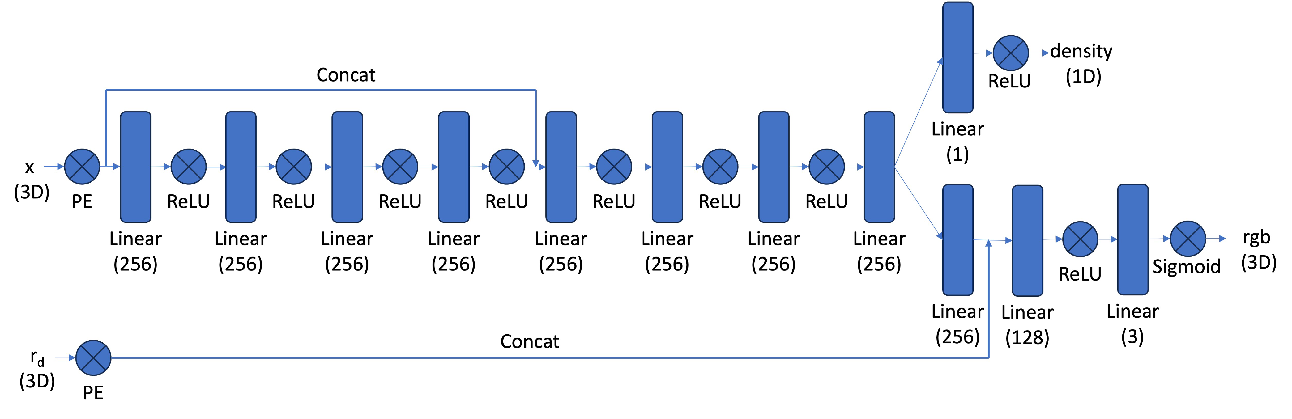
Network Architecture

We modified the neural network from Part 1 to handle 3D inputs instead of 2D. The network now predicts both the density and RGB color for each 3D point. Positional encoding was used for the 3D input coordinates and ray directions, with a reduced frequency for ray direction encoding. We made the MLP deeper and injected the positional encoding features of the input at intermediate layers to improve gradient flow and model capacity.

This part extends the neural field to 3D scenes using multi-view images. Rays are sampled from the images, and a volume rendering equation is applied to integrate densities and colors along the rays to generate pixel colors. Below is a diagram of the structure for the network implemented.

Camera and Ray Visualization

Below is the image of how the rays travel from the cameras through the images. The points are added to show how the rays sample points randomly on the rays and they are perturbed which we can see from the fact that the points are not spread out uniformly. The first image is a picture of rays from all cameras. The second image is rays from only one camera.

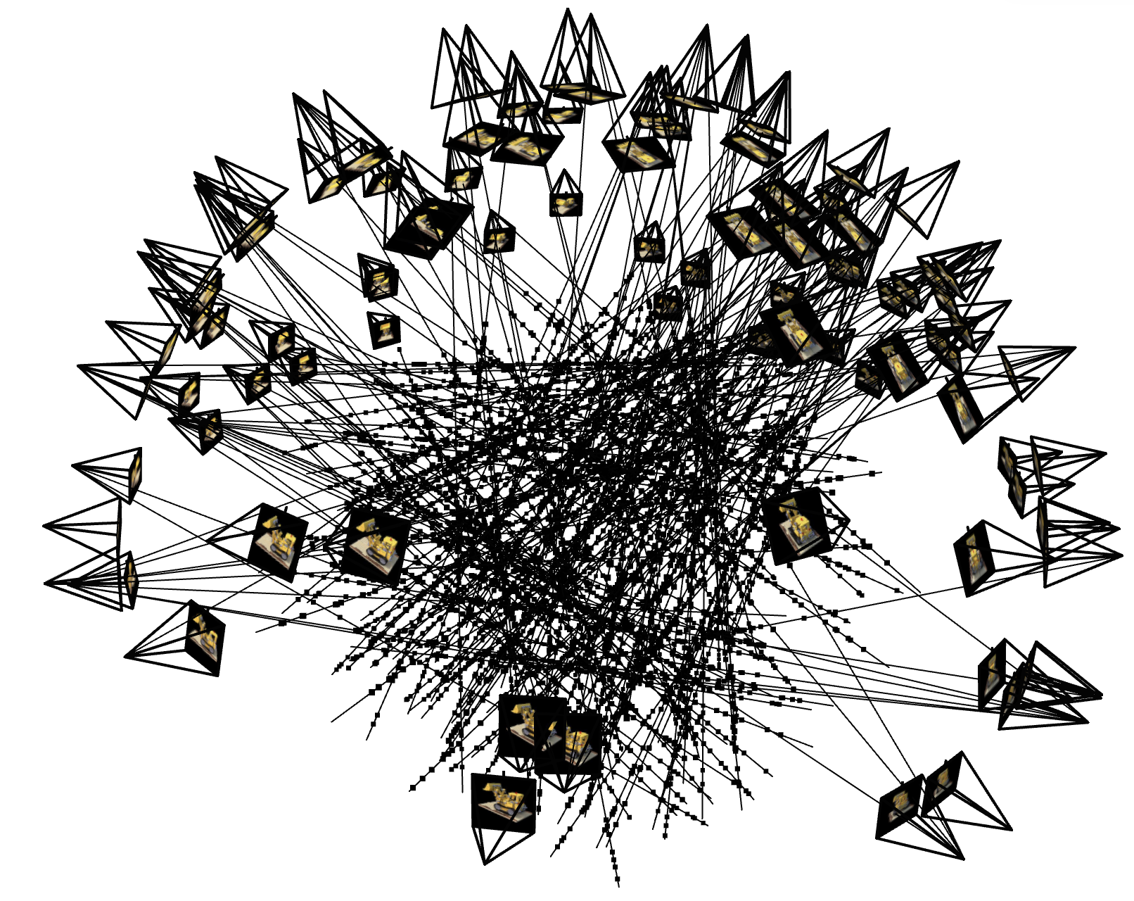
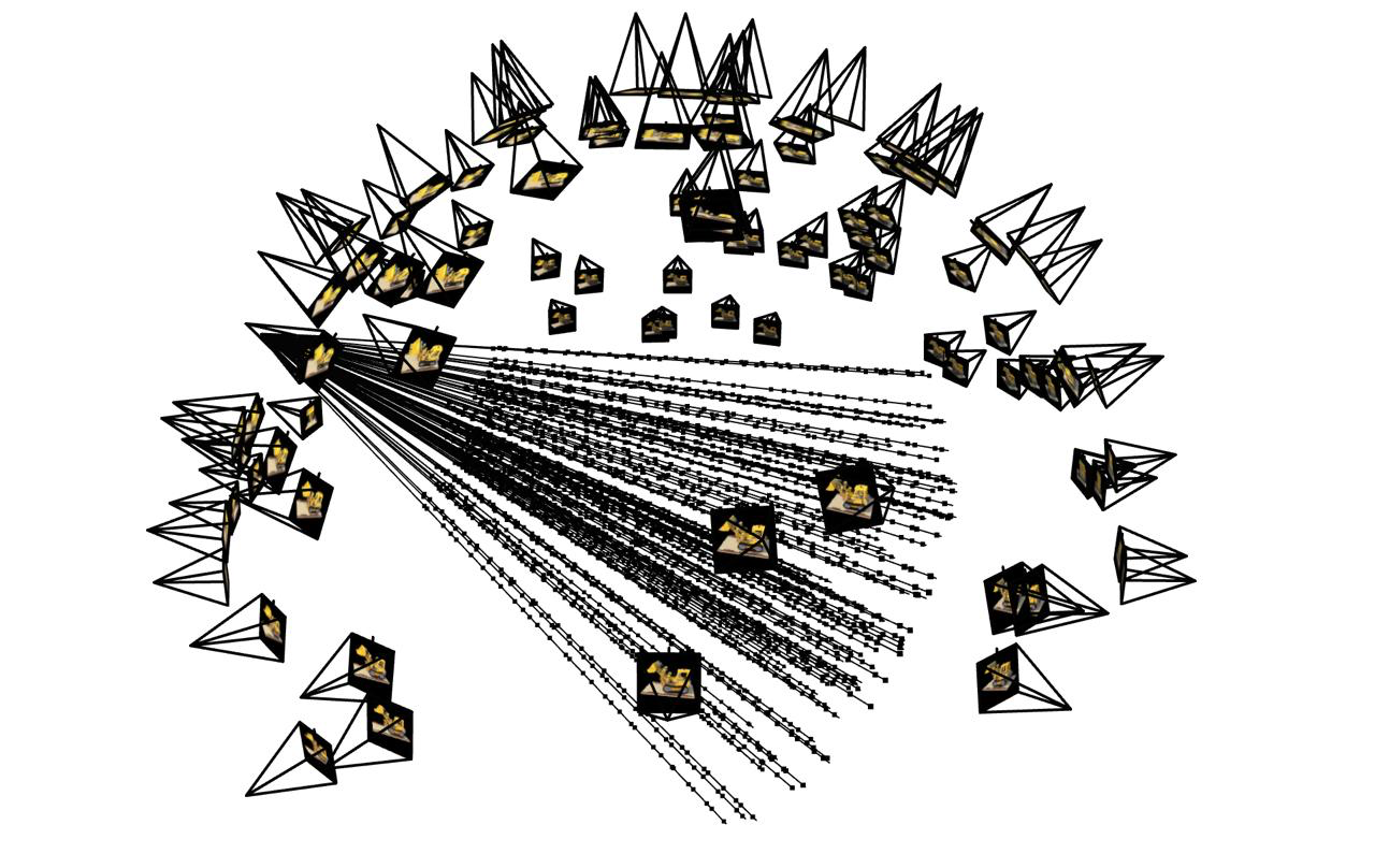
Visualization of sampled rays and camera frustums.

Volume Rendering Results

Progression of the rendered images during training. The image starts out blurry and becomes sharper as the model learns the scene.

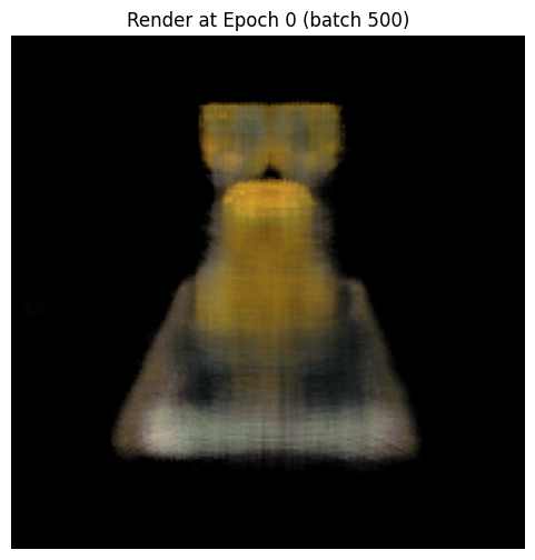
Epoch 0 Batch 500

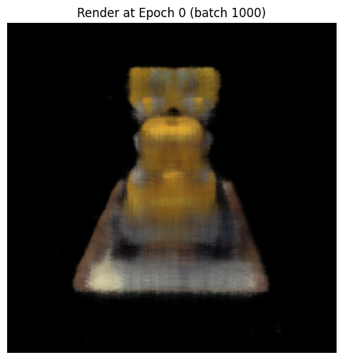
Epoch 0 Batch 1000

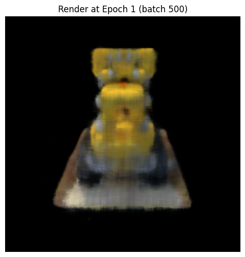
Epoch 1 Batch 500

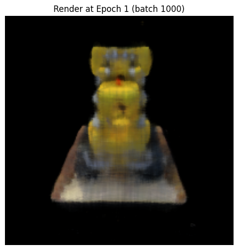
Epoch 1 Batch 1000

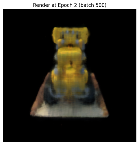
Epoch 2 Batch 500

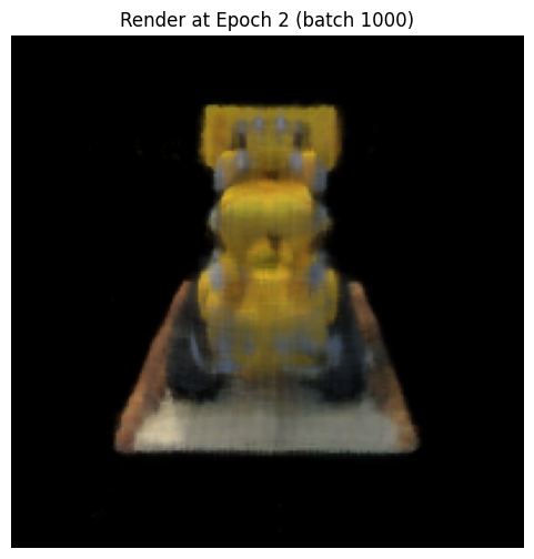
Epoch 2 Batch 1000

Here is the video of the final result of the 3D scene from both low resolution and high resolution. The high resolution had the following hyperparameters:

Number of positional encoding frequencies (L_x): 10
Number of directional encoding frequencies (L_r_d): 4
Hidden layer dimension: 256
RGB output dimension: 3
Density output dimension: 1
Number of hidden layers: 8

Low Resolution

High Resolution

PSNR Curve

As we can see from the plot below, the curve is rapidly increasing in the begninning and slowly converging to a high PSNR value of around 23-24 PSNR. Our final PSNR value was 23.6.

Plot showing the PSNR for validation images during training.

Bells and Whistles

For the B&W Portion, we added a blue background to the video by changing the volume function. The way we did this was by setting a threshold where if the transmittance was below a certain value, we would set the color to blue. This however, causes some aliasing issues as we can see which could have been fixed by implementing a solution where you add a color inverse proporsionally to the transmittance. Below is a video of the final result after 1 epoch given time contraints.

Custom Background Rendering

Acknowledgements

This project is part of CS 180 at UC Berkeley. Testing code and datasets were provided by course staff.